Assignment 4: Data structures and strings

In this assignment, you'll be adding functionality to the programs you wrote for Assignment 3, namely one_gram_reader.py, one_gram_plotter.py. There is a LOT in this assignment, so I've given way more hints than usual, particular during the tricky matplotlib parts. Do not feel like you should somehow know how to zip straight to the answer on these things. Do not feel shy at all about reading the hints.

In particular, we're going to study aggregate properties of the dataset, including the letter frequencies of English words, the distribution of word frequencies, and how the length of the average written word has changed since 1800.

Finish any labs that you haven't completed yet

As usual, before you begin this assignment: If you didn't finish the labs, you should complete those first. Labs can be found here.

Working with 1-grams

We'll be reusing the assignment 3 data files. As before, the 3 wfiles are "very_short.csv", "words_that_start_with_q.csv", and "all_words.csv", and you should use progressively move to larger files as you test your programs.

one_gram_reader

While the one_gram_reader we wrote for assignment 3 is perfectly fine for making plots of frequencies for particular words, it's not ideal since it only reads a small piece of the file into memory at once. As a result, we can't consider any aggregate properties of the dataset.

For the beginning of this assignment, you'll add a function called read_entire_wfile that will read in the entire 1gram dataset.

Your one_gram_reader module should contain the following functions:

def read_entire_wfile(wfile):            Returns the counts and years for all words
def read_wfile(word, year_range, wfile): Returns the counts and years for the word
def read_total_counts(tfile):            Returns the total number of words

read_entire_wfile(wfile)

Inputs:

wfile: A string giving the name of a one_gram csv file

Output:

word_data: A dictionary mapping from words to lists of tuples. For every word, there is exactly one list of tuples. Each tuple in this list represents a year in which a word appeared, in addition to the count of the number of times the word appeared that year. The year appears first in the tuple, and the count appears second. This is probably easier to understand from the example below.

Example:

word_data = read_entire_wfile("very_short.csv")
print(word_data)
print("----------------------------")
print(word_data["request"])

    
{'wandered': [(2005, 83769), (2006, 87688), (2007, 108634), 
(2008, 171015)], 'airport': [(2007, 175702), (2008, 173294)], 
'request': [(2005, 646179), (2006, 677820), (2007, 697645), 
(2008, 795265)]}
----------------------------
[(2005, 646179), (2006, 677820), (2007, 697645), (2008, 795265)]

Look carefully! Getting the format exactly is right is very important. For instance, observe that word_data maps the key "wandered" to a list of tuples. This list of tuples is 4 entries long, and every tuple contains exactly two items, and the first item in every tuple is the year, and the second is the number of occurrences of "wandered" in that year.

one_gram_plotter

Before proceeding, make sure you run test4.py on your one_gram_reader.read_entire_wfile function.

When you're done your one_gram_plotter.py module should contain the following functions. I've broken it up into three tasks. Feel free to skip any tasks that you don't want to do, as each is fully independent of the others. They are in order of roughly increasing difficulty. They will almost certainly take more than 6 hours to complete, so feel free to maybe come back and finish this in a future week if its taking forever.

def total_occurrences(word_data, word):             Returns total occurrences of word
def count_letters(word_data):                       Returns a list of length 26 corresponding to letter freqs
def bar_plot_of_letter_frequencies(word_data)       Plots frequencies of letters in English

Task 1: Plotting letter frequencies

def plot_aggregate_counts(word_data, words):        Plots distribution of word frequencies, and annotates words

Task 2: Plotting aggregate word counts

def get_occurences_in_year(word_data, word, year):  Gets number of occurrences of word during year specified
def get_average_word_length(word_data, year):       Gets the average length of all words from year specified
def plot_average_word_length(word_data, year_range):Make a plot of average word length of year range specified

Task 3: Plotting average word lengths vs. time

def normalize_counts(years, counts, total):         Returns the normalized count
def plot_words(words, year_range, wfile, tfile):    Plots the relative popularity of words over range specified

Assignment 3 tasks (already done)

Task 1: Plotting letter frequencies

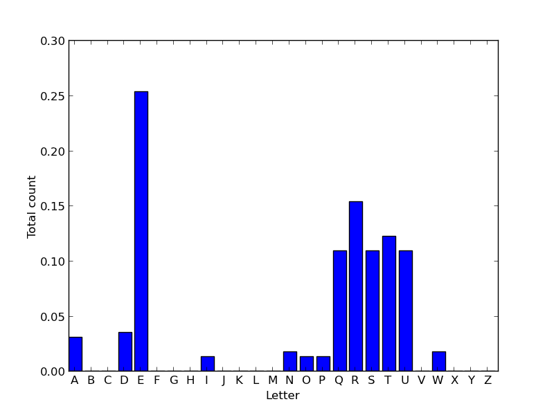
In this task, you'll create a plot of relative frequencies of letters in the English language. Along the way, you'll develop two helper functions that should give you some good practice with our new data structures.

total_occurrences(word_data, word)

Inputs:

word_data: A dictionary of word to tuples created by read_entire_wfile.
word: An english word. Not guaranteed to exist in word_data.

Outputs:

total_occurrences: The total number of times that a word has appeared in a book in the entire dataset.

Example:

import one_gram_reader
word_data = one_gram_reader.read_entire_wfile("very_short.csv")
print(total_occurrences(word_data, "wandered"))    
print(total_occurrences(word_data, "quetzalcoatl"))



451106
0

While somewhat interesting on its own, this function is primarily intended as a building block of the next function, count_letters.

count_letters(word_data):

Inputs:

word_data: A dictionary of word to tuples created by read_entire_wfile

Outputs:

letter_counts: A list of length 26 where the 0th element is the percentage of letters that are a, the 1st element is the percentage of letters that are b, and so forth.

Example:

import one_gram_reader word_data = one_gram_reader.read_entire_wfile("very_short.csv") print(word_data) print(count_letters(word_data))
{'wandered': [(2005, 83769), (2006, 87688), (2007, 108634), (2008, 171015)], 'airport': [(2007, 175702), (2008, 173294)], 'request': [(2005, 646179), (2006, 677820), (2007, 697645), (2008, 795265)]} [0.03104758705050717, 0.0, 0.0, 0.03500991824543893, 0.2536276129665047, 0.0, 0.0, 0.0, 0.013542627927787708, 0.0, 0.0, 0.0, 0.0, 0.017504959122719464, 0.013542627927787708, 0.013542627927787708, 0.10930884736053291, 0.15389906233882777, 0.10930884736053291, 0.12285147528832062, 0.10930884736053291, 0.0, 0.017504959122719464, 0.0, 0.0, 0.0]

In the example above, we get 0.03 by first counting the total number of as occurring in any word in any dictionary. We do this by noting that "wandered" and "airport" each contain exactly one a, and these words occur a total of (83769 + 87688 + 108634 + 171015 + 175702 + 173294) times. We divide this by the total number of letters in all words. To get the total number of letters, we observe that "wandered" is of length 8, "airport" is of length 7, and "request" is of length 7, and multiply each of these numbers by the total number of occurrences of each, e.g. 8 * (83769 + 87688 + 108634 + 171015).

You may find the letter counter function in lab 4 useful as a guide. Warning: if you use a dictionary in a manner similar to the lab, the letters may not appear in alphabetical order.

bar_plot_of_letter_frequencies(word_data):

Inputs:

word_data: A dictionary of word to tuples created by read_entire_wfile

Outputs: Returns nothing. Instead, creates a figure similar to that shown in the example.

Example:

import one_gram_reader
word_data = one_gram_reader.read_entire_wfile("very_short.csv")
bar_plot_of_letter_frequencies(word_data)

Your function should create a figure numbered 3. If figure 3 already exists, it should clear everything from the currently existing figure before drawing. Your graph should resemble the above graph as closely as possible. For this function, you'll be using the matplotlib.pyplot.bar function instead of matplotlib.pyplot.plot.

Below are some hints for some of the things you'll need to figure out. Highlight the hints to see them. Feel free to use the matplotlib gallery as a guide. If you're really stuck, check the solutions or post on piazza! It's not worth beating your head against the wall trying to find how to use the one magic command you need.

What do you use for the x-axis for the bar plot? Answer: A list of the integers from 0 to 25.
How do you set the labels on the x-axis? Answer: plt.gca().set_xticklabels()
How do you set the locations of the labels for the x-axis so that they're directly below each bar? I have too few labels or there aren't enough of them? Answer: The plt.gca().set_xticks() function will do the trick. You'll want to make sure the list you give to set_xticks is of length 26.

Task 2: Plotting aggregate word counts

plot_aggregate_counts(word_data, words):

Inputs:

word_data: A dictionary of word to tuples created by read_entire_wfile
words: A list of words to be annotated

Outputs: Returns nothing. Instead, creates a figure similar to that shown in the example.

Example:

import one_gram_reader
word_data = one_gram_reader.read_entire_wfile("words_that_start_with_the_letter_q.csv")
plot_aggregate_counts(word_data, ["quest", "questions"])

The x-axis is the rank of the word, where rank 1 is the most common word in English, rank 50 is the 50th most common word, and so forth. The y-axis is the total number of occurrences in all books in the database. Conveniently, that total_occurrences for Task 1 works perfectly for this purpose.

Your function should create a figure numbered 4. If figure 4 already exists, it should clear everything from the currently existing figure before drawing. This time, you'll be using matplotlib.pyplot.loglog instead of matplotlib.pyplot.plot. It is not important that you match the colors shown. You should match the marker shapes, however.

More hints:

Do not attempt to do everything at once! You should just get the basic shape right before trying to get all the little doodads correct.
What list should I use for the y data? Answer: A list L where L[0] is the total number of occurrences of the rank 1 word in English, L[1] the rank 2 word in English, and so forth.
How do I create that list? Answer: Given a list of the frequencies of all words in English, you can sort them using the built in list sorting function. Since you want them in decreasing order, you'll also want to reverse this list.
How do I make the axes tight around my data? Matplotlib keeps leaving empty space on the side! Answer: plt.gca().autoscale_view(tight=True, scalex=True, scaley=True) will do the trick. How would you know that? Stackoverflow or by looking at the matplotlib gallery.
How do I plot data as dots or stars? Answer: Simply put a third argument into the plot function, e.g. plt.plot(x, y, "*") plots data as discrete stars instead of as a connected line.
How do I make the markers bigger? Answer: Add a 4th argument to your calls to any plotting function that sets ms equal to some number, e.g. plt.plot(x, y, "*", ms = 12).
How do I plot the same data as dots AND lines? Answer: Just call plot with the same data twice, but without a marker specification one of those times. The one that you put second will get put on top of the other.
How do I figure out the coordinates for my stars from the words? It seems like sorting the frequencies scrambles everything up and I don't know where the word I want went; this seems very hard! Answer: Yep, it's actually pretty damn tricky. The key is to realize that you know the total number of occurrences of the word in question. For example, if you know "potato" occurs 43,512 times, you can use the list function called index to look up where potato occurs. This now gives you the location where potato ended up after sorting. This is probably the trickiest thing on the whole assignment. Don't forget to use a try/except in case the word in question isn't in the list at all.
How do I get text on my graph? Answer: Use the matplotlib.pyplot.annotate function. See the gallery or look at the solutions for the optional part of assignment 3 for an example.
The text on my graph is overlapping the line and it looks ugly. What should I do? Answer: Consider multiplying your x and y coordinates by a small constant factor to scoot the text over a bit.

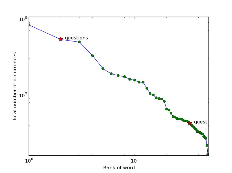
Now that you've got a nice plot, you might notice something very odd. Look carefully, and you'll see that on this loglog plot, word rank vs. total number of occurrences seems to follow a power law -- i.e. it looks to be a roughly straight line with some negative slope. The sudden drop-off on the right hand side is almost certainly an artifact of the technique I used to cut off the full 4 gigabyte database to a more manageable size.

This observation of a power law relationship between word occurrence and word rank is known as Zipf's law. Intriguingly, nobody really knows why "it holds for most languages".

Task 3: Plotting average word lengths vs. time

get_occurrences_in_year(word_data, word, year):

Inputs:

word_data: A dictionary of word to tuples created by read_entire_wfile
word: A string representing an English word. The word does not necessarily appear in word_data
year: An integer representing the year of interest

Outputs:

total_occurrences: An integer giving the total number of occurrences of the word during the year specified.

Example:

import one_gram_reader word_data = one_gram_reader.read_entire_wfile("very_short.csv") print(word_data) print(get_occurrences_in_year(word_data, "wandered", 2007))
{'wandered': [(2005, 83769), (2006, 87688), (2007, 108634), (2008, 171015)], 'airport': [(2007, 175702), (2008, 173294)], 'request': [(2005, 646179), (2006, 677820), (2007, 697645), (2008, 795265)]} 108634

You should use this function as a building block for constructing the next function, get_average_word_length.

get_average_word_length(word_data, year):

Inputs:

word_data: A dictionary of word to tuples created by read_entire_wfile
year: An integer representing the year of interest

Outputs:

average_length: A floating point number representing the average length of all words during the year specified.

Example:

import one_gram_reader word_data = one_gram_reader.read_entire_wfile("very_short.csv") print(word_data) print(get_average_word_length(word_data, 2006))
{'wandered': [(2005, 83769), (2006, 87688), (2007, 108634), (2008, 171015)], 'airport': [(2007, 175702), (2008, 173294)], 'request': [(2005, 646179), (2006, 677820), (2007, 697645), (2008, 795265)]} 7.1

To arrive at the answer, we observe that in 2006, the word "wandered" appears 87,688 times and is of length 8, the word "airport" appears 0 times, and the word "request" appears 677,820 times and is of length 7. This results in an average length of 7.1 letters.

plot_average_word_length(word_data, year_range):

Inputs:

word_data: A dictionary of word to tuples created by read_entire_wfile
year_range: A list (or tple) of two numbers representing the desired date range

Outputs: Returns nothing. Instead, creates a figure similar to that shown in the example.

Example:

import one_gram_reader
word_data = one_gram_reader.read_entire_wfile("words_that_start_with_q.csv")
plot_average_word_length(word_data, [1860, 1880])

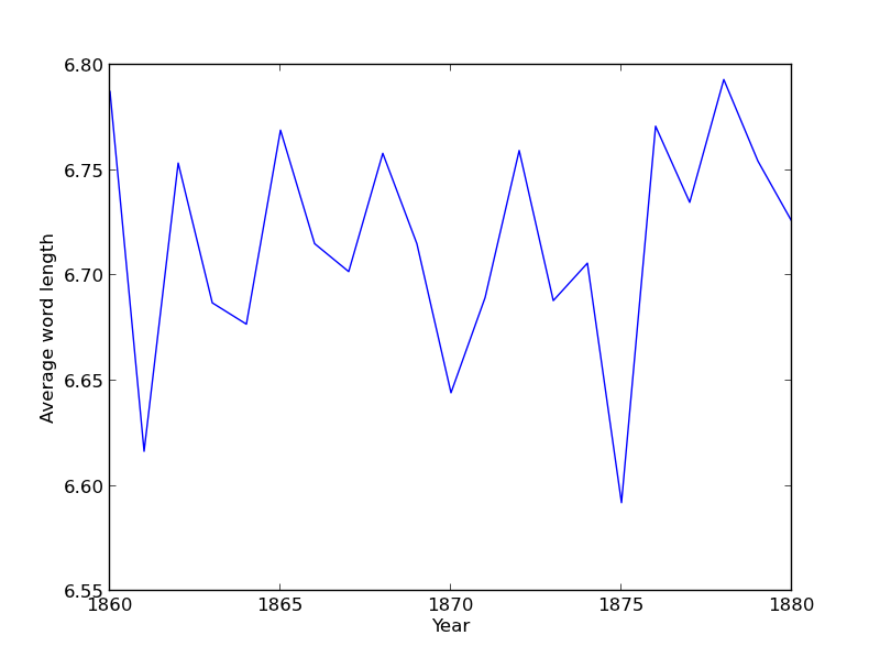
I've intentionally stuck to this tiny range and restricted dataset (words that start with q) so that you can discover the (rather surprising!) results for yourself using the full data set and date range.

Your function should create a figure numbered 5. If figure 5 already exists, it should clear everything from the currently existing figure before drawing.