For this assignment, you'll be using CSV files and Matplotlib to explore the relative frequency of English words over time. We'll also be getting a sneak preview of a new data structure called a dictionary that we'll be going over in much more detail next week.
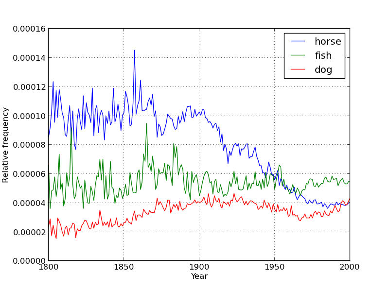
When you're done, you should end up with two python files called one_gram_reader.py and one_gram_plotter.py. Together, these modules will be able to generate plots like the following, which shows the relative popularity of the words horse, fish, and dog between 1800 and 2000.
An Ngram is a sequence of N contiguous items. Types of items include letters, syllables, words, base-pairs, amino acids, etc. Given a text, we can count all of the 1grams, 2grams, 3grams, etc that appear in the text. The N refers to the number of items in the Ngram.
For example, if the items of interest are words, the set of 2-grams for this sentence is: {For example, example the, the set, set of, of 2-grams, 2-grams for, for this, this sentence, sentence is:}. If we were interested in letters instead, the 2-grams would be {Fo, or, r , e, ex, xa, am, mp, pl, ...}. Some of these 2-grams appear more than once. For example, the 2gram th appears 3 times.
Ngram frequencies are useful because they provide a quantitative measure of which items tend to follow others in a certain data domain. For example, the list of 2-grams from all English texts is likely to include "robotic dog", but it probably does include "robotic noodle".
Ngrams are used heavily in statistical processing of natural languages or other strings. For example, you can use Ngram frequencies to identify what language a particular text comes from. Similarly, you can use them to identify which species a given sequences comes from.
For this assignment you'll be working with only 1grams. Given a text, and assuming we care about the words (as opposed to the letters, or syllables, or whatever else), the set of 1grams is just the set of words that appear in the text.
As part of Google's book scanning project, they've collected the frequencies of all 1, 2, 3, 4, and 5grams that appear in all English books they've analyzed. All of that time you've spent filling out captchas is finally about to pay off.
For this assignment, you will be writing two modules to deal with one_grams. The first is one_gram_reader.py, which will have two functions that each process a distinct type of CSV file. The first function will read a word CSV-file and return the number of times that a given word has appeared throughout history. For example, the word "wandered" appeared 108634 times during the year 2007. The second function will read a total CSV-file and return the total number of words collected from all sources. For example, Google counted a total of 16,206,118,071 English words in 2007. We'll call these files wfiles and tfiles throughout this assignment.
The second module you'll write is one_gram_plotter.py, which will use the data provided by one_gram_reader to track the relative popularity of words over time.
Before you start, you'll need to download the assignment 3 data files. This zip file includes 3 wfiles and 1 tfile. Each of the wfiles is a subset of Google's 1gram file, which is just a wee bit too big for you guys to download (clocking in at around 4 gigabytes of zipfiles). For the curious, these were compiled using this script. The 3 wfiles are "very_short.csv", "words_that_start_with_q.csv", and "all_words.csv". You should use progressively move to larger files as you test your programs.
For more context on Google Ngrams, see this interview.
Your one_gram_reader module should contain the following functions:
def read_wfile(word, year_range, wfile):          Returns the counts and years for the word
def read_total_counts(tfile):                     Returns the total number of words
years, counts = read_wfile("request", [2005, 2007], "very_short.csv")
print(years)
print(counts)
|
[2005, 2006, 2007]
[646179, 677820, 697645] |
This function should read in the wfile provided and return two lists. You may assume that the wfile file is a tab separated csv file with the format as shown below.
airport     2007    175702  32788
airport     2008    173294  31271
request     2005    646179  81592
request     2006    677820  86967
request     2007    697645  92342
request     2008    795265  125775
wandered    2005    83769   32682
wandered    2006    87688   34647
wandered    2007    108634  40101
wandered    2008    171015  64395
The first entry in each row is the word. The second entry is the year. The third entry is the the number of times that the word appeared in any book that year. The fourth entry is the number of distinct sources that contain that word. Your program should ignore this fourth column. For example, from the text file above, we can observe that the word wandered appeared 171,015 times during the year 2008, and these appearances were spread across 64,395 distinct texts.
Your function should return empty lists if the word does not appear in the CSV file in the date range specified. All entries outside the data range specified should be ignored. In the example above, the desired date range is only from 2005 to 2007, and hence the 2008 appearance of "request" is disregarded.
You should use the CSV exercise in the lab as a guide. It is important that you specify a delimiter. In this case, since the file is tab separated, your delimiter should be '\t'.
total_counts = read_total_counts("total_counts.csv")
print(total_counts[1507])
print(total_counts[1525])
|
49576
3359 |
This function should read in the tfile provided and return a dictionary of total word counts. A dictionary is sort of like a list, and is explained further down this page. You may assume that the tfile is a comma separated csv file with the format as shown below:
1505,32059,231,1
1507,49586,477,1
1515,289011,2197,1
1520,51783,223,1
1524,287177,1275,1
1525,3559,69,1
The first entry in each row is the year. The second is the total number of words recorded from all texts that year. The third number is the total number of pages of text from that year. The fourth is the total number of distinct sources from that year. Your program should ignore the third and fourth numbers. For example, we see that Google has exactly one text from the year 1505, and that it contains 32,059 words and 231 pages.
As mentioned above, your function will return a dictionary instead of a list. We'll discuss dictionaries in full detail next week, but for now, I'll explain by example. Consider the following list based program:
some_list = [] some_list[1508] = "puppy chow" |
IndexError: list assignment index out of range |
It crashes because we're trying to modify the 1,508th element of the list, but it doesn't have that many entries. We could get around this by creating a big empty list that contains at least 1508 entries, for example, we could use one of the following two equivalent solutions.
some_list = [0] * 1600 some_list[1508] = "puppy chow" | some_list = []
for i in range(1600):
some_list.append(0)
some_list[1508] = "puppy chow" |
If you're wondering what's going on with multiplying a list by 1600, we mentioned towards the beginning of class on week 3 that this is a thing you can do with lists. If you missed it, don't fret, it's just the same thing as writing a for loop that appends 0 to a list 1600 times. While either of these approaches work, creating a list with tons of useless entries is a rather inelegant solution. As a preview of next week's class, we'll be using a more elegant solution known in Python as a dictionary (a.k.a. an associative array, map, or symbol table). The equivalent dictionary code is as follows:
some_list = {}
some_list[1508] = "puppy chow"
|
Look carefully! The difference is simply in how the dictionary is created. Instead of using brackets [], we use curly brackets {}. We're going to spend an entire day on this stuff next week, so for now, just accept that if you use curly brackets, you don't have to create a big empty list. For our purposes, everything else is exactly the same -- though if you try printing the dictionary, you'll see that the underlying structure is a bit more complicated. Try it!
Before proceeding, make sure you run test3.py on your one_gram_reader.
Your one_gram_plotter.py module should contain the following functions:
def normalize_counts(years, counts, total):         Returns the normalized count
def plot_words(words, year_range, wfile, tfile):    Plots the relative popularity of words over range specified
import one_gram_reader
years, counts = one_gram_reader.read_wfile("request", [2000, 2010], "very_short.csv")
total = one_gram_reader.read_total_counts("total_counts.csv")
print(years)
first_observed_year = years[0]
print(first_observed_year)
print(counts[0])
print(total[first_observed_year])
normalized_counts = normalize_counts(years, counts, total)
print(normalized_counts[0])                                #equal to 646179 / 14425183957
|
[2005, 2006, 2007, 2008]

2005
646179
14425183957

4.47951999729e-05
|
This is a utility function that will help you when you're working on your plot_words function. The idea is that knowing the absolute number of times that "requested" appeared in a given year is not very useful for tracking the popularity of a word over time. This is because there are relatively few books from long ago, and thus all English words are likely to increase in usage over time.
Example:
plot_words(["horse", "fish", "dog"], [1800, 2000], "all_words.csv", "total_counts.csv") |
Your function should create a figure numbered 1. If figure 1 already exists, it should clear everything from the currently existing figure before drawing. Your x-axis and y-axis should be labeled. You should also include a legend and there should be a grid over your plot.
Useful functions that you should use:
If you want to save your figure to a file, you can use plt.savefig("somefile.png").
plot_words(["horse", "fish"], [1800, 2000], "all_words.csv", "total_counts.csv") |
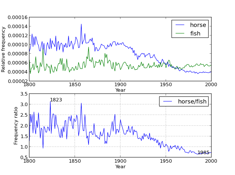
Your function should create a figure numbered 2. If figure 2 already exists, it should clear everything from the currently existing figure before drawing. The top subfigure should be exactly as in plot_words. The bottom subfigure should display the ratio of the relative popularity of the two words. Your x-axes and y-axes should be labeled. Both subfigures should have legends as shown. The years with maximum and minimum ratio should be annotated in the bottom subfigure.
To calculate the ratio, you might consider converting the lists to numpy arrays, as unlike lists, it is possible to divide one numpy array by another.